
Tensorflow2 learning note (2)
In the second part of this Tensorflow2 mini-series, I will write about how to make use of the pre-trained and well-established deep learning models to perform new tasks. Still, the note serves as a template of the modeling pipeline instead of a sophisticated performance-oriented project. Keras applications has provided a list of deep learning models having the top performance on the ImageNet image recognition tasks with pre-trained weights, and those models can be used for predictions, feature extraction, and fine-tuning. In the post, I will first use the ResNet50 model and its pre-trained weights to classify a dog image, then use the VGG19 model to perform a transfer learning task where features from the last MaxPooling2D layer of the VGG19 are served as the starting point of a logistic regression classifying dogs vs cats. The dataset I used in the post is a subset from Kaggle’s Dogs vs. Cats. In addition, I am glad that my dog bro Dandan has granted permission to use one of his photos as the test data.
The post mainly consists of four parts,
- Use ResNet50 to classify the test image
- Explore features learned by each layer of VGG19
- Load image dataset and use ImageDataGenerator to perform data augmentation
- Use VGG19 layers + new layers to train a logistic regression model
and details are given below. The work is originally created on Google Colab with GPU processor.
1. Use ResNet50 to classify the test image
# import the modules

import tensorflow as tf
print(tf.__version__)

from tensorflow.keras import Input, layers
from tensorflow.keras.models import  Sequential, Model
from tensorflow.keras.preprocessing import image

import os
import numpy as np
import pandas as pd
import matplotlib.pyplot as plt
%matplotlib inline

import IPython.display as display
# from PIL import Image
from IPython.display import Image
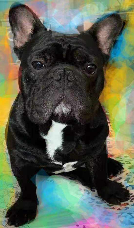
The test image is a photo of Dandan with the face a bit grumpy.
# display the test image

img_path = '/content/drive/MyDrive/Colab Notebooks/dog.jpeg'
# display.display(Image.open(img_path))
Image(img_path, width=80, height=200 )
# import the ResNet50 image processing functions and instantiate the ResNet50 model

from tensorflow.keras.applications.resnet50 import preprocess_input, decode_predictions
model_resnet50 = tf.keras.applications.ResNet50(weights='imagenet')
The default input shape of the ResNet50 model is (224, 224, 3), and we need to use the model-specific data processing functions to process the images.
img_path = '/content/drive/MyDrive/Colab Notebooks/dog.jpeg'

# load image to target size
img = image.load_img(img_path, target_size=(224, 224))

# convert image to numpy arrays
x = image.img_to_array(img)

# expand image dimension to (batch, width, height, depth)
x = np.expand_dims(x, axis=0)

# use resnet50.preprocess_input to process the image
x = preprocess_input(x)

# take the top 5 predictions and decode them to the corresponding labels
x_preds = decode_predictions(model_resnet50.predict(x), top=5)
Voila! The ResNet50 is 99.84% confident that Dandan is a French bulldog, and he is! Interestingly, ImageNet has 120 dog breeds classes and also there is a Kaggle competition dedicated on the Dog Breed identification using the canine subset of the ImageNet, so next time when you come across a cute doggy on the road but don’t know its breed, instead of searching on Google, using ResNet50 or other deep learning models might give you some clue about the breed!
# print the top 5 predictions

df = pd.DataFrame([list(x[1:3]) for x in x_preds[0]],columns=['Class','Probability'])
print(df.to_string(index = False))
                     Class  Probability
            French_bulldog     0.998435
                       pug     0.000937
               Boston_bull     0.000487
         Brabancon_griffon     0.000069
 Staffordshire_bullterrier     0.000011
2. Explore the features learned by each layer of VGG19
As I was learning the deep learning models, I found it’s difficult to imagine what each layer is learning, but the good news is that we can actually visualize the output of each layer, which would give us some idea about the learning process. The VGG19 model is trained on the ImageNet dataset and has 26 layers, and by default the output layer gives a vector of size 1,000 as the image representative features. In this section, I will explore the features generated from the 2nd and the 11th layer of VGG19.
# instantiate VGG19 model

from tensorflow.keras.applications import VGG19
model_vgg19 = VGG19(weights='imagenet')
# print out model summary
# model_vgg19.summary()

# plot the model architecture
# tf.keras.utils.plot_model(model_vgg19, 'model_vgg19.png', show_shapes=True)

# print the number of layers
print("The number of layers in VGG19 is", len(model_vgg19.layers))
The number of layers in VGG19 is 26
In order to get the output from each layer, we need to use the keras.models functional API Model(), instead of the sequential API used in the part 1 of the notes. We specify the input of the VGG19 as the model inputs, and the outputs from all the layers as the model outputs.
# store the layers outputs of VGG19
outputs_vgg19 = [layer.output for layer in model_vgg19.layers]

# use functional API to instantiate a new model
features_vgg19 = Model(inputs=model_vgg19.input, outputs=outputs_vgg19)

# process the image data
x = image.img_to_array(img)
x = np.expand_dims(x, axis=0)
x = tf.keras.applications.vgg19.preprocess_input(x)

# get features generated by all layers of the VGG19
x_features = features_vgg19(x)
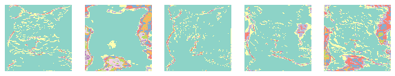
The layer index starts from 0. The second layer of VGG19 has output shape (224, 224, 64), and I randomly select 5 channels from the last dimension and display them below. It can be observed that at this stage, the model is roughly learning about the shape of the object in an image.
# features from the second layer

features_layer1 = x_features[1][0]
ran_idx = np.random.choice(features_layer1.shape[-1], size=5, replace=False)

plt.figure(figsize=(10,10))
for i,n in enumerate(ran_idx):
  ax = plt.subplot(1,5,i+1)
  plt.imshow(features_layer1[:,:,n], cmap='Set3')
  plt.axis('off')
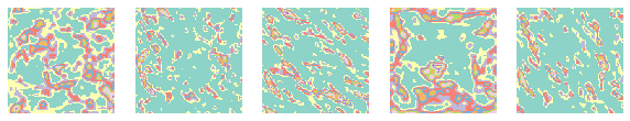
The 11th layer has output shape (56, 56, 256). Similarly, I randomly select 5 channels from the last dimension and display them below. It looks like at this layer, the model is learning about the local information around the shape of the object.
# features from the 11th layer

features_layer10 = x_features[10][0]
ran_idx = np.random.choice(features_layer10.shape[-1], size=5, replace=False)

plt.figure(figsize=(10,10))
for i,n in enumerate(ran_idx):
  ax = plt.subplot(1,5,i+1)
  plt.imshow(features_layer10[:,:,n], cmap='Set3')
  plt.axis('off')
3. Load Dogs vs. Cats images and Data Augmentation
For the following sections, I will show how to construct a transfer learning model to classify dog vs. cat. Here I only use a subset (600 train, 300 test) of the dataset from Kaggle’s Dogs vs. Cats, if you are interested in how to import and process the initial data, you can refer to this article.
images_train = np.load('/content/drive/MyDrive/Colab Notebooks/image_data/images_train.npy')
images_test = np.load('/content/drive/MyDrive/Colab Notebooks/image_data/images_test.npy')

labels_train = np.load('/content/drive/MyDrive/Colab Notebooks/image_data/labels_train.npy')
labels_test = np.load('/content/drive/MyDrive/Colab Notebooks/image_data/labels_test.npy')
# display some sample images

ran_idx = np.random.choice(images_train.shape[0], size=5, replace=False)

plt.figure(figsize=(10,10))
for i,n in enumerate(ran_idx):
  ax = plt.subplot(1,5,i+1)
  plt.imshow(images_train[n,]/255.0)
  plt.axis('off')

If the train set and test set are large, it’s recommended to use the data/image generators. Since generators will only load the batch of data when it’s called instead of loading all the batches at once, it will reduce the memory cost. Moreover, keras has provided the generator class ImageDataGenerator() which not only converts the dataset into a generator but can also perform data augmentation. Generally speaking, data augmentation helps increase the training size by transforming the images into different versions, thus has the potential to increase the model performance. What the generator of ImageDataGenerator() does is to transform the train images to different versions at each training epoch, and it does not directly increase the train size1.
# define how to transform the train image

img_train_generator = image.ImageDataGenerator(
    # process the image as required by VGG19
    preprocessing_function=tf.keras.applications.vgg19.preprocess_input,

    # rotate
    rotation_range=120,

    # brightness
    brightness_range=(0.5, 1.5),

    # flip
    horizontal_flip=True)


# do not do any transformation on the test data
img_test_generator = image.ImageDataGenerator(
    preprocessing_function=tf.keras.applications.vgg19.preprocess_input
)

# need to fit first if there is sample statistics used in the augmentation, like mean, sd etc.
# img_train_generator.fit(images_train)

# instantiate the generator
train_generator = img_train_generator.flow(images_train, labels_train, batch_size = 32, shuffle=False)
test_generator = img_test_generator.flow(images_test, labels_test, batch_size=32, shuffle=False)
4. Transfer learning
In this section I will use the pre-trained weights and the flattened output from the last MaxPooling2D layer of the VGG model as the input features, and add a new Dense layer with one unit and sigmoid activation to construct a logistic regression model. There are two things need to pay attention to. (1) The default input shape the VGG19 is (224, 224, 3), while the train data has input shape (160, 160, 3), therefore we need to assign a new input shape for the model. (2) If we want to use the pre-trained weights from VGG19, we do not need to train it in the new model, hence set the attribute trainable of VGG19 layers to False.
# reset the input shape to (160, 160, 3)
model_vgg19_newhead = VGG19(weights='imagenet', include_top=False,
                            input_tensor = Input(shape=(160,160,3)))

# do not train the vgg19 weights in the new model
for layer in model_vgg19_newhead.layers:
  layer.trainable = False

# flatten the output from the last layer and set it as input feature of new model
h = model_vgg19_newhead.layers[-1].output
h = tf.keras.layers.Flatten()(h)

# add dense layer to perform logistic regression
outputs = tf.keras.layers.Dense(1, activation='sigmoid')(h)

# instantiate the model
model_vgg19_transfer = Model(inputs=model_vgg19_newhead.input, outputs = outputs)

# print out model summary
model_vgg19_transfer.summary()
Downloading data from https://storage.googleapis.com/tensorflow/keras-applications/vgg19/vgg19_weights_tf_dim_ordering_tf_kernels_notop.h5
80142336/80134624 [==============================] - 0s 0us/step
Model: "model_1"
_________________________________________________________________
Layer (type)                 Output Shape              Param #
=================================================================
input_3 (InputLayer)         [(None, 160, 160, 3)]     0
_________________________________________________________________
block1_conv1 (Conv2D)        (None, 160, 160, 64)      1792
_________________________________________________________________
block1_conv2 (Conv2D)        (None, 160, 160, 64)      36928
_________________________________________________________________
block1_pool (MaxPooling2D)   (None, 80, 80, 64)        0
_________________________________________________________________
block2_conv1 (Conv2D)        (None, 80, 80, 128)       73856
_________________________________________________________________
block2_conv2 (Conv2D)        (None, 80, 80, 128)       147584
_________________________________________________________________
block2_pool (MaxPooling2D)   (None, 40, 40, 128)       0
_________________________________________________________________
block3_conv1 (Conv2D)        (None, 40, 40, 256)       295168
_________________________________________________________________
block3_conv2 (Conv2D)        (None, 40, 40, 256)       590080
_________________________________________________________________
block3_conv3 (Conv2D)        (None, 40, 40, 256)       590080
_________________________________________________________________
block3_conv4 (Conv2D)        (None, 40, 40, 256)       590080
_________________________________________________________________
block3_pool (MaxPooling2D)   (None, 20, 20, 256)       0
_________________________________________________________________
block4_conv1 (Conv2D)        (None, 20, 20, 512)       1180160
_________________________________________________________________
block4_conv2 (Conv2D)        (None, 20, 20, 512)       2359808
_________________________________________________________________
block4_conv3 (Conv2D)        (None, 20, 20, 512)       2359808
_________________________________________________________________
block4_conv4 (Conv2D)        (None, 20, 20, 512)       2359808
_________________________________________________________________
block4_pool (MaxPooling2D)   (None, 10, 10, 512)       0
_________________________________________________________________
block5_conv1 (Conv2D)        (None, 10, 10, 512)       2359808
_________________________________________________________________
block5_conv2 (Conv2D)        (None, 10, 10, 512)       2359808
_________________________________________________________________
block5_conv3 (Conv2D)        (None, 10, 10, 512)       2359808
_________________________________________________________________
block5_conv4 (Conv2D)        (None, 10, 10, 512)       2359808
_________________________________________________________________
block5_pool (MaxPooling2D)   (None, 5, 5, 512)         0
_________________________________________________________________
flatten (Flatten)            (None, 12800)             0
_________________________________________________________________
dense (Dense)                (None, 1)                 12801
=================================================================
Total params: 20,037,185
Trainable params: 12,801
Non-trainable params: 20,024,384
_________________________________________________________________
As can be seen from the model summary, only 12,801 parameters are trainable, the rest of the parameters belong to the VGG19 model and are set not to be trained. Next we compile and train the new model for 10 epochs, then evaluate it on the test set. The result shows that the test accuracy is 100%.
# compile the model
model_vgg19_transfer.compile(optimizer='RMSprop',
                 loss='binary_crossentropy',
                 metrics=['accuracy'])

# train the model for 10 epochs
history = model_vgg19_transfer.fit(
    train_generator, epochs=10,
    # number of batches for each epoch
    steps_per_epoch=train_generator.n // train_generator.batch_size,
    verbose=0)

# evaluate on the test set
test_loss, test_acc = model_vgg19_transfer.evaluate(
    test_generator,
    steps = test_generator.batch_size // test_generator.batch_size,
    verbose=0)

# print out the test result
print("Test loss: {}".format(test_loss))
print("Test accuracy: {}".format(test_acc))
Test loss: 0.02071295864880085
Test accuracy: 1.0
Now we test the new model on classifying the photo of Dandan, and it successfully predicts that Dandan is a dog!
img = image.load_img('/content/drive/MyDrive/Colab Notebooks/dog.jpeg', target_size=(160, 160))

x = image.img_to_array(img)
x = np.expand_dims(x, axis=0)
x = tf.keras.applications.vgg19.preprocess_input(x)
if model_vgg19_transfer.predict(x)<0.5:
  print('Yes, Model predicts that Dandan is a dog')
else:
  print('Oops, Model predicts that Dandan is a cat')
Yes, Model predicts that Dandan is a dog
5. Other reference articles
Difference between numpy array shape (R,1) and (R,)
Control trainable parameters in transfer learning
Why set include_top=False when input shape is not the default in transfer learning