
Tensorflow2 learning note (1)
Recently I have been taking a series of online courses to learn Tensorflow2, simply out of curiosity to know how it works, especially nowadays when almost everyone is talking about AI, deep learning, etc. 😛. In the post, I will show how to build up a neural network model from scratch to classify images of human-written digits of 0 to 9. This is the part 1 of the Tensorflow2 mini-series, and it serves more like a template demonstrating the modeling pipeline than a sophisticated performance-oriented project. I just randomly set up the model architecture, and the accuracy of the test dataset using the trained neural network model is 97.91%. Some models on Kaggle can achieve test accuracy more than 99.00%, those are also good resources to learn how to process the image data and improve the model performance.
Personally, on one hand I feel amazed that deep learning models can achieve such impressive performance superior than the other traditional statistical or machine learning models such as support vector machine (SVM) or random forest (RF). However, on the other hand I can sense that the real challenge resides on (1) how to adjust the model structure or refine the data processing to increase the accuracy by 1%, 0.1% or just 0.01%? (2) understand what pattern/relationship the model has learned from the data? As for the first challenge, it seems to me that it would require professional experience and extensive experiments, those classical models available on Keras Applications do not look very intuitive. The second challenge is related to an emerging research area called interpretable machine learning1 2, and I have heard from a machine learning engineer working in a pharmaceutical company that they use graph neural networks (GNN) to understand the connections between the molecule structure of drugs and their properties. Those are definitely very interesting topics, I will explore more on them and hopefully I will be able to cover the topics in my blog in the future 🤔.
The simple modeling pipeline presented in the post mainly consists of four parts,
- Load modules and data
- Construct model and specify training algorithm & evaluation metrics
- Train model using train set and set up stopping criteria
- Evaluate model performance on test set
and details are displayed below. The work is originally created on Google Colab with GPU processor.
1. Load modules and Tensorflow2
Instead of installing Tensorflow2 on local computer, it’s more convenient to use Google Colab, which can import Tensorflow2 directly and specify faster GPU option. Here the Colab default Tensorflow2 version is 2.x and I set the working directory to a folder in the Google Drive.
import tensorflow as tf
print('Tensorflow2 version', tf.__version__)

from tensorflow.keras.models import Sequential
from tensorflow.keras.layers import (Dense, Flatten, Conv2D, MaxPooling2D,
                                     Softmax, Dropout, BatchNormalization)
from tensorflow.keras.preprocessing import image
from tensorflow.keras import regularizers

import numpy as np
import pandas as pd
import matplotlib.pyplot as plt
%matplotlib inline
Tensorflow2 version 2.4.1
# set working directory

% cd /content/drive/MyDrive/Colab Notebooks
/content/drive/MyDrive/Colab Notebooks
2. Load Data
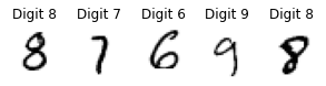
The MINST data can be loaded from Keras and is splitted into train set (60,000) and test set (10,000). I scale the image data to be in the range [0,1] and append a dummy third dimension, since the convolutional layer expects three dimensions. Some examples of the digit images and their corresponding labels are given below.
# load the MNIST Digits data
mnist_data = tf.keras.datasets.mnist
(train_images, train_labels), (test_images, test_labels) = mnist_data.load_data()

# scale images to be in range [0,1]
train_images_scale, test_images_scale = train_images/255.0, test_images/255.0

# add dummy channel dimension
train_images_scale = train_images_scale[...,np.newaxis]
test_images_scale = test_images_scale[...,np.newaxis]

print("train_images_scale shape:", train_images_scale.shape)
print("test_images_scale shape:", test_images_scale.shape)
train_images_scale shape: (60000, 28, 28, 1)
test_images_scale shape: (10000, 28, 28, 1)
# example images and labels

random_idx = np.random.choice(train_images_scale.shape[0],size=5)

fig, axes = plt.subplots(1,5,figsize=(5,5))

for i, idx in enumerate(random_idx):
  axes[i].set_axis_off()
  axes[i].imshow(np.squeeze(train_images_scale[idx]), cmap='Greys')
  axes[i].set_title(f'Digit {train_labels[idx]}')
3. Build and Compile model
I use model Sequential API to build up a neural network model of seven layers, and there is no specific rationals regarding the configuration, simply for fun 😎. Note that the last Dense layer is set to have 10 units, since there are 10 digit classes. When compiling the model, specify Adam as the training algorithm, loss is calculated by sparse_categorical_crossentropy, and model performance is measured by SparseCategoricalAccuracy. Then instantiate my_model from the defined model class and the summary is displayed below to show the layers structure and the number of parameters involved.
def get_model(input_shape):

  # specify layers
  model = Sequential([
    Conv2D(filters=16, kernel_size=(3,3), strides=(2,2),
           padding='SAME', activation='relu',
           input_shape=input_shape, data_format='channels_last',
           # Conv2D expects (batch_size,dim,dim,channels);
           # specify the channel axis accordingly in data_format
           name = "layer_1"),
    MaxPooling2D(pool_size=(3,3), name="layer_2"),
    Flatten(name="layer_3"),
    Dense(units=128, activation = 'relu', kernel_regularizer=regularizers.l2(1e-4),
          name="layer_4"),
    Dense(units=64, activation = 'relu', kernel_initializer='he_uniform',
          bias_initializer=tf.keras.initializers.Constant(value=0),
          kernel_regularizer=regularizers.l2(1e-4),
          name="layer_5"),
    BatchNormalization(name="layer_6"),
    Dense(units=10, activation = 'softmax',
          kernel_initializer=tf.keras.initializers.RandomNormal(mean=0.0, stddev=0.05),
          bias_initializer="zeros",
          kernel_regularizer=regularizers.l2(1e-4),
          name="layer_7")
    ])

  # compile model
  model.compile(optimizer=tf.keras.optimizers.Adam(learning_rate=0.001),
                loss='sparse_categorical_crossentropy',
                metrics=[tf.keras.metrics.SparseCategoricalAccuracy()])

  return model

# instantiate model
my_model = get_model(train_images_scale[0].shape)

# display the model summary
my_model.summary()
Model: "sequential"
_________________________________________________________________
Layer (type)                 Output Shape              Param #
=================================================================
layer_1 (Conv2D)             (None, 14, 14, 16)        160
_________________________________________________________________
layer_2 (MaxPooling2D)       (None, 4, 4, 16)          0
_________________________________________________________________
layer_3 (Flatten)            (None, 256)               0
_________________________________________________________________
layer_4 (Dense)              (None, 128)               32896
_________________________________________________________________
layer_5 (Dense)              (None, 64)                8256
_________________________________________________________________
layer_6 (BatchNormalization) (None, 64)                256
_________________________________________________________________
layer_7 (Dense)              (None, 10)                650
=================================================================
Total params: 42,218
Trainable params: 42,090
Non-trainable params: 128
_________________________________________________________________
Before training the model, we first check the model performance using the initial weights. The test accuracy is 7.82%.
def get_test_evaluate(model, x, y):

  test_loss, test_acc = model.evaluate(x, y, verbose=0)
  print("Test loss: {:.3f}\nTest accuracy: {:.2f}%".format(test_loss, 100 * test_acc))

get_test_evaluate(my_model, test_images_scale, test_labels)
Test loss: 2.335
Test accuracy: 7.82%
4. Train model
mode.fit() method is used to train the neural network model for 50 epochs and 15% of the training set is set aside as validation set. Note that there are many helpful callback classes we can make use of to manipulate the training process. For examples, we set callbacks_early_stop to tell the machine to stop updating if the validation loss is not improved for 3 consecutive epochs; checkpoints_best tells the machine to save the best model weights in terms of the validation loss; checkpoints_epoch makes the machine save the model weights after each epoch. The results from the first 5 epochs are given below.
# stop if val_loss stops improving for 3 consecutive epochs
callbacks_early_stop = tf.keras.callbacks.EarlyStopping(monitor='val_loss', mode='min', patience=3)

# reduce learning rate by a factor 0.5 if val_loss stops improving for 3 consecutive epochs
callbacks_reduce_lr = tf.keras.callbacks.ReduceLROnPlateau(factor=0.5, patience=3)

# save the loss and metrics after each epoch in the .csv file
callbacks_csv = tf.keras.callbacks.CSVLogger("train_results.csv")

# save the model weights after each epoch
checkpoints_epoch = tf.keras.callbacks.ModelCheckpoint(filepath='checkpoints_epoch/checkpoints_{epoch:03d}',
                                                       frequency='epoch', save_weights_only=True, verbose=0)

# save the best model weights in terms of the lowest val_loss
checkpoints_best = tf.keras.callbacks.ModelCheckpoint(filepath='checkpoints_best/checkpoints_best',
                                                       frequency='epoch', save_weights_only=True, verbose=0,
                                                      save_best_only = True, monitor='val_loss')

# train 50 epochs, and split 15% data as validation set
history = my_model.fit(train_images_scale, train_labels,
                       epochs=50, batch_size = 128, validation_split=0.15, verbose=0,
                       callbacks=[callbacks_early_stop, callbacks_reduce_lr, callbacks_csv,
                                  checkpoints_epoch, checkpoints_best])
# check the training metrics, which is also saved in the train_results.csv
df = pd.DataFrame(history.history)
df.head()
| loss | sparse_categorical_accuracy | val_loss | val_sparse_categorical_accuracy | lr | |
|---|---|---|---|---|---|
| 0 | 0.438134 | 0.899392 | 0.225271 | 0.953444 | 0.001 |
| 1 | 0.130286 | 0.968392 | 0.164475 | 0.953111 | 0.001 |
| 2 | 0.101795 | 0.977137 | 0.119016 | 0.971222 | 0.001 |
| 3 | 0.086796 | 0.980922 | 0.118879 | 0.971667 | 0.001 |
| 4 | 0.077237 | 0.983980 | 0.119780 | 0.972778 | 0.001 |
5. Evaluate model performance
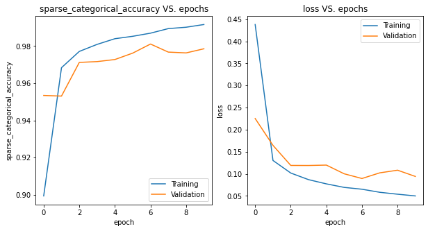
We now visualize how the model performance changes as the number of training epochs increases. As shown from the plot, the loss and accuracy of both training and validation sets are decreasing and increasing, respectively. However, the loss and accuracy of validation set are worse than those of training set, which implies there is the overfitting issue. One may consider conducting data augmentation to increase the training size or adding regularizations to the weights.
fig = plt.figure(figsize=(10,5))

fig.add_subplot(121)
plt.plot(history.history['sparse_categorical_accuracy'])
plt.plot(history.history['val_sparse_categorical_accuracy'])
plt.title('sparse_categorical_accuracy VS. epochs')
plt.ylabel('sparse_categorical_accuracy')
plt.xlabel('epoch')
# plt.xticks(np.arange(epochs))
plt.legend(['Training', 'Validation'], loc='lower right')

fig.add_subplot(122)
plt.plot(history.history['loss'])
plt.plot(history.history['val_loss'])
plt.title('loss VS. epochs')
plt.ylabel('loss')
plt.xlabel('epoch')
# plt.xticks(np.arange(epochs))
plt.legend(['Training', 'Validation'], loc='upper right')

plt.show()

print('After model fitting:')
get_test_evaluate(my_model, test_images_scale, test_labels)
After model fitting:
Test loss: 0.096
Test accuracy: 97.70%
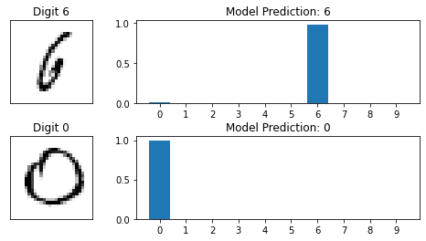
In addition, we evaluate the trained model on the test set and obtain the test accuracy 97.70%, which has dramatically increased from 7.82%, the value before model training. Moreover, we randomly select two test images and use the trained model to make predictions as well as the corresponding bar plot. It looks like the test images are clear and the model gives pretty good predictions 🥳.
# select two test images
random_idx = np.random.choice(test_images_scale.shape[0], size=2)
random_images = test_images_scale[random_idx, ...]
random_labels = test_labels[random_idx, ...]

# make predictions
random_predictions = my_model.predict(random_images)

# plot
fig, axes = plt.subplots(2, 2, figsize = (10,4))
fig.subplots_adjust(hspace = 0.4, wspace = -0.2)

for i, (pred, image, label) in enumerate(zip(random_predictions, random_images, random_labels)):

  axes[i,0].imshow(np.squeeze(image), cmap='Greys')
  axes[i,0].get_xaxis().set_visible(False)
  axes[i,0].get_yaxis().set_visible(False)
  axes[i,0].set_title(f'Digit {label}')
  axes[i,1].bar(np.arange(len(pred)), pred)
  axes[i,1].set_xticks(np.arange(len(pred)))
  axes[i,1].set_title(f'Model Prediction: {np.argmax(pred)}')

plt.show()
6. Load model weights and architecture
As mentioned in section 4, we have set up some callbacks to save the model weights after each epoch and the best model weights of all epochs. Here we check the performances of model using weights from the last epoch and the best weights, respectively. It shows that test accuracy of model using the best weight is higher, with value 97.91%.
# build up models with same layers structure
new_model_last = get_model(train_images_scale[0].shape)
new_model_best = get_model(train_images_scale[0].shape)

# load the weights from the last epoch
new_model_last.load_weights(tf.train.latest_checkpoint('checkpoints_epoch'))

# load the best weights
new_model_best.load_weights('checkpoints_best/checkpoints_best')

print('Use weights from last epoch:')
get_test_evaluate(new_model_last, test_images_scale, test_labels)
print('\nUse weights from best epoch:')
get_test_evaluate(new_model_best, test_images_scale, test_labels)
Use weights from last epoch:
Test loss: 0.096
Test accuracy: 97.70%

Use weights from best epoch:
Test loss: 0.087
Test accuracy: 97.91%
The model.load_weights() method is very useful in the scenario where one needs to stop then resume the training process. Method model.load_model() can be called if one wants to load a pre-trained model including both model architecture and weights. Furthermore, If one wants to extract the model configuration, method model.get_config() will retrieve the config in dictionary format, and it’s also possible to obtain the config in JSON or YAML format.
# extract model architecture
config_dict = my_model.get_config()

# load model architecture
new_model_config = tf.keras.Sequential.from_config(config_dict)
# for models that are not sequential models, use tf.keras.Model.from_config()