As a statistician, I use R a lot in my school works and collaboration projects, since R provides almost all the statistical analysis tools I would need in my research, from data wrangling, statistical modeling, simulation, to data visualization. Normally statisticians/biostatisticians would employ R to implement and publish their latest statistical techniques, so using R makes it convenient to follow up those up to date developments. However, sometimes I did find out that Python is faster than R when they perform the same task as data size goes larger, for example, when using K-means model and spectral clustering model. There are also many articles online comparing the speed of Python and R in various scenarios. Therefore, it might be a good idea to combine Python and R together to make use of the good parts from both worlds.

reticulate is a R package which calls Python from R in a variety of ways including R Markdown, sourcing Python scripts, importing Python modules, and using Python interactively within an R session. In the post, I will present a simple example of microarray analysis, where spectral clustering model is imported from Python to cluster genes into different groups and graphical tools are called in R to display the clustering results. By the end, I will also demonstrate how to transfer data between R and Python.

1. Import data

I use the gene expression data from a study on brewer’s yeast cells. The data has 378 samples and 5900 genes and is already normalized¹ by the provider. First transform the data into a matrix of 378 rows and 5900 columns, then standardize columns such that each column has mean zero and unit variance.

#load data
gene_df <- read.delim("GSE75694_matrix_378_samples.txt")
dim(gene_df)
# 5900  379

gene_names <- gene_df$ID_REF %>% as.character()
sample_names <- colnames(gene_df)
gene_mat <- gene_df[,2:ncol(gene_df)] %>% as.matrix()
gene_mat <- t(gene_mat)
colnames(gene_mat) <- NULL
rownames(gene_mat) <- NULL

# standardize columns
gene_scale <- scale(gene_mat) 

2. Import Python modules

One can call Python by either specifying a path or a Conda environment (need to install anaconda). Here I choose to create a Conda environment, and import modules numpy and sklearn.cluster.

# install and load R package reticulate
install.packages('reticulate')
library(reticulate) 

# check and create an anaconda working environment
conda_list()
conda_create("r-reticulate")
use_condaenv("r-reticulate", required = TRUE)

# check python configuration
py_config()

# install packages
conda_install('r-reticulate', packages = c('numpy','pandas'), channel = 'conda-forge')
conda_install('r-reticulate', packages = 'scikit-learn', channel = 'conda-forge')

# import packages
numpy <- import('numpy')
sklearn_cluster <- import('sklearn.cluster')

3. Spectral clustering

Spectral clustering model is used to cluster the genes into 20 groups and the group labels will be saved. When fitting the model, the absolute correlation matrix of the standardized genes is set as the affinity matrix and the number of clusters is 20. Note that the indexing system in Python starts from 0, while the indexing system in R starts from 1. Most importantly, when the arguments of Python functions require integer, we need explicitly specify the integer property in R, i.e. use ‘20L’ instead of ‘20’, otherwise, error will occur. After fitting the model, we can take a look at the frequencies of the 20 clustered groups.

# absolute correlation as affinity matrix
gene_scale_abscor <- r_to_py(abs(cor(gene_scale)))
# r_to_py() is not necessary
# reticulate package will take care of the transformation between R data and Python data

# cluster 5900 genes into 20 groups
# !!! specify the integer L
spec_model <- sklearn_cluster$SpectralClustering(n_clusters=20L, affinity="precomputed")
spec_fit <- spec_model$fit(X=gene_scale_abscor)

# save the labels
spec_label <- spec_fit$labels_+1

# frequency of each group
table(spec_label)
# spec_label
#   1   2   3   4   5   6   7   8   9  10  11  12  13  14  15  16  17  18  19  20 
# 274 203 289 235 392 258 853 356 272 305 211 265 167 397 140 231 364 190 334 164 

4. Heatmap

In order to visualize the group structure, we display the heatmap of the correlation matrix using the R package ComplexHeatmap. Before making the plot, we define a helper function to rearrange the columns and rows of the correlation matrix according to their group memberships.

# helper function
reorder_col <- function(label, K){

  order_vec <- vector()
  for (k in c(1:K)){
    order_vec <- c(order_vec, which(label==k))
  }

  return(order_vec)
}

# rearrange the columns by groups
col_by_label <- reorder_col(spec_label, K=20)

# get correlation matrix
gene_scale_cor <- cor(gene_scale)

# install and load package
install.packages('ComplexHeatmap')
suppressPackageStartupMessages(library(ComplexHeatmap))

# plot heatmap 
Heatmap(
  gene_scale_cor, 
  
  cluster_rows = FALSE, cluster_columns = FALSE,
  show_row_names = FALSE, show_column_names = FALSE,
  
  column_order = col_by_label,
  row_order = col_by_label,
  
  show_heatmap_legend = TRUE,
  heatmap_legend_param = list(
    title = "gene correlation", 
    title_position = "leftcenter-rot",
    legend_height = unit(3, "cm")
  ),
  
  column_title = "Standardized Gene Expression \n Correlation Matrix K=20",
  use_raster = TRUE,
  raster_resize = FALSE, 
  raster_device = "CairoPNG"
)

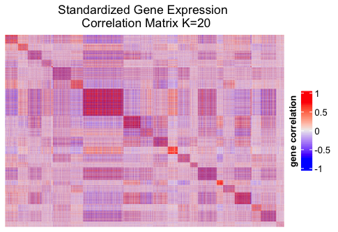
From the heatmap we can observe that the correlation matrix has a clear group structure. Further analysis needs to be conducted to explore the characteristics of the genes of different groups.

Some other clustering models might require the genes to follow certain distribution, for example, the Gaussian mixture model assumes the data follows normal distributions. A simple visual check on the genes densities can be done by plotting the density heatmap as below. On the left figure, we plot the densities of the first 50 genes in group 1, and on the right figure we compare the densities of 50 columns following the standard normal distribution.

# create a matrix with 50 columns following N(0,1)
rnorm_mat = matrix(rnorm(378*50), nrows=378)

# density plot
ht_list = densityHeatmap(gene_scale[,which(spec_label==1)[1:50]],
                         ylim = c(-2,2),
                         title = 'Density of Genes in Group 1 (N=50)',
                         ylab = 'Density',
                         heatmap_legend_param = list(title = "density")
) + densityHeatmap(scale(rnorm_mat),
                   ylim = c(-2,2),
                   title = 'Density of N(0,1)',
                   ylab = '',
                   heatmap_legend_param = list(title = "N(0,1) density"),
                   show_heatmap_legend = TRUE
)

draw(ht_list)

5. Transfer data between Python and R

Package reticulate will convert R data type to the corresponding Python data type and vice versa in R environment, but sometimes one may still need to transfer data between R and Python. In this case, we can use feather package. For example, we save the clustering labels spec_label in R then load it in Python.

## save data in R as .feather
install.packages('feather')
library('feather')

write_feather(spec_label, "spec_label_R.feather")

## load R data in Python
import feather

spec_label_Python = feather.read_dataframe("spec_label_R.feather")
feather.write_dataframe(spec_label_Python, "spec_label_Python.feather")

## load Python data in R

read_feather("spec_label_Python.feather")